
 数据结构
数据结构 网络
网络 RDBMS
RDBMS 操作系统
操作系统 Java
Java iOS
iOS HTML
HTML CSS
CSS Android
 Python
 C 编程
C 编程 C++
C++ C#
C# MongoDB
 MySQL
MySQL Javascript
 PHP
PHP使用 Python 的 Pandas 分析 TRAI 的移动数据速度
在本教程中,我们将利用 pandas 包分析移动数据速度。从TRAI 官方网站下载移动速度。下载文件步骤。
算法
1. Go to the [TRAI](https://myspeed.trai.gov.in/ ) website.
2. Scroll down to the end of the page.
3. You will find mobile speed data for different months.
4. Download the September mobile data speeds.
我们来看看CSV 文件中的列。
网络名称
网络技术
测试类型
速度
信号强度
状态
我们需要pandas、numpy、matpoltlib 库。让我们开始编码以分析数据。
示例
# importing requires libraries
import pandas as pd
import numpy as np
import matplotlib.pyplot as plot
# constants
DATASET = 'sept19_publish.csv'
NETWORK_NAME = 'JIO'
STATE = 'Andhra Pradesh'
# lists to store the values
download_speeds = []
upload_speeds = []
states = []
operators = []
# importing the dataset using pandas
data_frame = pd.read_csv(DATASET)
# assigning column names for easy access
data_frame.columns = ['Network', 'Technology', 'Type Of Test', 'Speed', 'Signal Str
ength', 'State']
# getting unique states and operators from the dataset
unique_states = data_frame['State'].unique()
unique_operators = data_frame['Network'].unique()
print(unique_states)
print()
print(unique_operators)
输出
如果您运行以上的程序,您将获得以下结果。
['Kolkata' 'Punjab' 'Delhi' 'UP West' 'Haryana' nan 'West Bengal'
'Tamil Nadu' 'Kerala' 'Rajasthan' 'Gujarat' 'Maharashtra' 'Chennai'
'Madhya Pradesh' 'UP East' 'Karnataka' 'Orissa' 'Andhra Pradesh' 'Bihar'
'Mumbai' 'North East' 'Himachal Pradesh' 'Assam' 'Jammu & Kashmir']
['JIO' 'AIRTEL' 'VODAFONE' 'IDEA' 'CELLONE' 'DOLPHIN']
继续...
# getting the data related to one network that we want
# we already declared the network previously
# this filtering the data
JIO = data_frame[data_frame['Network'] == NETWORK_NAME]
# iterating through the all states
for state in unique_states:
   # getting all the data of current state
   current_state = JIO[JIO['State'] == state]
   # getting download speed from the current_state
   download_speed = current_state[current_state['Type Of Test'] == 'download']
   # calculating download_speed average
   download_speed_avg = download_speed['Speed'].mean()
   # getting upload speed from the current_state
   upload_speed = current_state[current_state['Type Of Test'] == 'upload']
   # calculating upload_speed average
   upload_speed_avg = upload_speed['Speed'].mean()
   # checking if the averages or nan or not
   if pd.isnull(download_speed_avg) or pd.isnull(upload_speed_avg):
      # assigning zeroes to the both speeds
      download_speed, upload_speed = 0, 0
   else:
      # appending state if the values are not nan to plot
      states.append(state)
   download_speeds.append(download_speed_avg)
   upload_speeds.append(upload_speed_avg)
   # printing the download ans upload averages
   print(f'{state}: Download Avg. {download_speed_avg:.3f} Upload Avg. {upload _speed_avg:.3f}')
输出
如果您运行以上代码,您将获得以下结果。
Kolkata: Download Avg. 31179.157 Upload Avg. 5597.086
Punjab: Download Avg. 29289.594 Upload Avg. 5848.015
Delhi: Download Avg. 28956.174 Upload Avg. 5340.927
UP West: Download Avg. 21666.673 Upload Avg. 4118.200
Haryana: Download Avg. 6226.855 Upload Avg. 2372.987
West Bengal: Download Avg. 20457.976 Upload Avg. 4219.467
Tamil Nadu: Download Avg. 24029.364 Upload Avg. 4269.765
Kerala: Download Avg. 10735.611 Upload Avg. 2088.881
Rajasthan: Download Avg. 26718.066 Upload Avg. 5800.989
Gujarat: Download Avg. 16483.987 Upload Avg. 3414.485
Maharashtra: Download Avg. 20615.311 Upload Avg. 4033.843
Chennai: Download Avg. 6244.756 Upload Avg. 2271.318
Madhya Pradesh: Download Avg. 15757.381 Upload Avg. 3859.596
UP East: Download Avg. 28827.914 Upload Avg. 5363.082
Karnataka: Download Avg. 10257.426 Upload Avg. 2584.806
Orissa: Download Avg. 32820.872 Upload Avg. 5258.215
Andhra Pradesh: Download Avg. 8260.547 Upload Avg. 2390.845
Bihar: Download Avg. 9657.874 Upload Avg. 3197.166
Mumbai: Download Avg. 9984.954 Upload Avg. 3484.052
North East: Download Avg. 4472.731 Upload Avg. 2356.284
Himachal Pradesh: Download Avg. 6985.774 Upload Avg. 3970.431
Assam: Download Avg. 4343.987 Upload Avg. 2237.143
Jammu & Kashmir: Download Avg. 1665.425 Upload Avg. 802.925
继续...
# plotting the graph'
fix, axes = plot.subplots()
# setting bar width
bar_width = 0.25
# rearranging the positions of states
re_states = np.arange(len(states))
# setting the width and height
plot.figure(num = None, figsize = (12, 5))
# plotting the download spped
plot.bar(re_states, download_speeds, bar_width, color = 'g', label = 'Avg. Download
Speed')
# plotting the upload speed
plot.bar(re_states + bar_width, upload_speeds, bar_width, color='b', label='Avg. Up
load Speed')
# title of the graph
plot.title('Avg. Download|Upload Speed for ' + NETWORK_NAME)
# x-axis label
plot.xlabel('States')
# y-axis label
plot.ylabel('Average Speeds in Kbps')
# the label below each of the bars,
# corresponding to the states
plot.xticks(re_states + bar_width, states, rotation = 90)
# draw the legend
plot.legend()
# make the graph layout tight
plot.tight_layout()
# show the graph
plot.show()
输出
如果您运行以上的图表,您将获得以下图表。
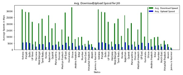
结论
根据您的需要,您可以绘制不同的图表。通过绘制不同的图表来使用该数据集。如果您对本教程有任何疑问,可以在评论部分中提到。

更新时间: 2020 年 7 月 8 日
94 次浏览

广告