
 数据结构
数据结构 网络
网络 关系型数据库管理系统 (RDBMS)
 操作系统
操作系统 Java
Java iOS
iOS HTML
HTML CSS
CSS Android
 Python
 C语言编程
C语言编程 C++
C++ C#
C# MongoDB
 MySQL
MySQL Javascript
 PHP
PHP使用PyTorch实现深度自编码器进行图像重建
机器学习是人工智能的一个分支,它涉及开发能够使计算机从输入数据中学习并做出决策或预测的统计模型和算法,而无需硬编码。它涉及使用大型数据集训练机器学习算法,以便机器能够识别数据中的模式和关系。
什么是自编码器?
具有自编码器的神经网络架构用于无监督学习任务。它由编码器和解码器网络组成,这些网络经过训练可以重建输入数据,方法是将其压缩成低维表示(编码),然后对其进行解码以恢复其原始形式。
为了鼓励网络学习数据的有价值的特征或表示,目标是最小化输入和输出之间的重建误差。自编码器的突出应用包括数据压缩、图像去噪和异常检测。这减少了与数据传输相关的许多工作和成本。
在本文中,我们将探讨如何使用PyTorch的深度自编码器进行图像重建。这个深度学习模型将使用MNIST手写数字进行训练,在学习输入图像的表示后,它将重建数字图像。一个基本的自编码器包含两个主要功能:
编码器
解码器
编码器接收输入,并通过一系列层将高维数据转换为相同值的潜在低维表示。解码器使用此潜在表示,使用Python库torch、PyTorch工作流程中的torchvision库以及numpy和matplotlib等通用库来生成重建数据。
算法
导入所有必需的库。
初始化将应用于获得的数据集的每个条目的转换操作。
由于Pytorch需要张量才能运行,因此我们首先将每个项目转换为张量并对其进行归一化,以保持像素值在0到1之间的范围。
使用torchvision.datasets程序下载数据集,并分别将其保存在./MNIST/train和./MNIST/test文件夹中,用于训练集和测试集。
为了加快学习速度,将这些数据集转换为批量大小等于64的数据加载器。
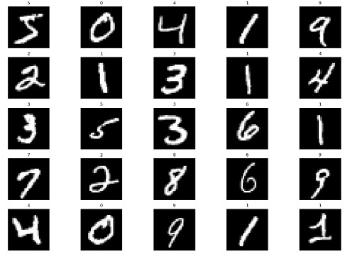
随机打印集合中的25张照片,以便我们更好地理解正在处理的信息。
步骤1:初始化
此步骤涉及导入所有必要的库,例如numpy、matplotlib、pytorch和torchvision。
语法
torchvision.transforms.ToTensor():
将输入图像(以PIL或numpy格式)转换为PyTorch张量格式。此转换还将像素强度从[0, 255]范围缩放为[0, 1]。
torchvision.transforms.Normalize(mean, std)
使用均值和标准差值对输入图像张量进行归一化。此转换有助于提高深度学习模型在训练期间的收敛速度。均值和标准差值通常是从训练数据集中计算出来的。
torchvision.transforms.Compose(transforms)
允许将多个图像转换链接到单个对象中。此对象可以传递给PyTorch Dataset对象,以便在训练或推理期间动态应用转换。
示例
#importing modules
import numpy as np
import matplotlib.pyplot as plt
import torch
from torchvision import datasets, transforms
plt.rcParams['figure.figsize'] = 15, 10

# Initialize the transform operation
transform = torchvision.transforms.Compose([
   torchvision.transforms.ToTensor(),
   torchvision.transforms.Normalize((0.5), (0.5))
])

# Download the inbuilt MNIST data
train_dataset = torchvision.datasets.MNIST(
   root="./MNIST/train", train=True,
   transform=torchvision.transforms.ToTensor(),
   download=True)
test_dataset = torchvision.datasets.MNIST(
   root="./MNIST/test", train=False,
   transform=torchvision.transforms.ToTensor(),
   download=True)
输出
步骤2:初始化自编码器
我们首先初始化Autoencoder类,它是torch.nn.Module的子类。由于这为我们抽象了许多样板代码,因此我们现在可以专注于创建我们的模型架构,如下所示:
语法
torch.nn.Linear()
一个将线性变换应用于输入张量的模块。
my_linear_layer = nn.Linear(in_features, out_features, bias=True)
torch.nn.ReLU()
一个将修正线性单元 (ReLU) 函数应用于输入张量的激活函数。
torch.nn.Sigmoid()
一个将sigmoid函数应用于输入张量的激活函数。
示例
#Creating the autoencoder classes
class Autoencoder(torch.nn.Module):
   def __init__(self):
      super().__init__()
      self.encoder=torch.nn.Sequential(
         torch.nn.Linear(28*28,128), #N, 784 -> 128
         torch.nn.ReLU(),
         torch.nn.Linear(128,64),
         torch.nn.ReLU(),
         torch.nn.Linear(64,12),
         torch.nn.ReLU(),
         torch.nn.Linear(12,3), # --> N, 3
         torch.nn.ReLU()
      )

      self.decoder=torch.nn.Sequential(
         torch.nn.Linear(3,12), #N, 3 -> 12
         torch.nn.ReLU(),
         torch.nn.Linear(12,64),
         torch.nn.ReLU(),
         torch.nn.Linear(64,128),
         torch.nn.ReLU(),
         torch.nn.Linear(128,28*28), # --> N, 28*28
         torch.nn.Sigmoid()
      )

   def forward(self,x):
      encoded=self.encoder(x)
      decoded = self.decoder(encoded)
      return decoded

# Instantiating the model and hyperparameters
model = Autoencoder()
criterion = torch.nn.MSELoss()
num_epochs = 10
optimizer = torch.optim.Adam(model.parameters(), lr=1e-3)
步骤3:创建训练循环
我们正在训练一个自编码器模型来学习图像的压缩表示。训练循环总共遍历数据集10次。
为每批图像迭代计算模型的输出。
然后计算输出图像和原始图像之间的质量差异。
它平均每批的损失,并存储每个 epoch 的图像及其输出。
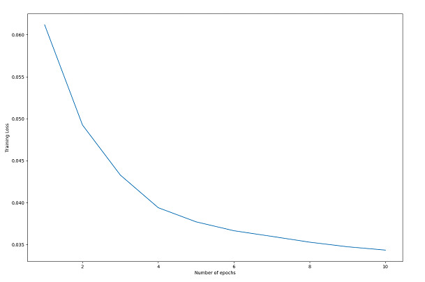
循环完成后,我们绘制训练损失,以帮助理解训练过程。
该图显示损失随着每个 epoch 的推移而降低,这表明模型正在学习新的信息,并且训练过程是成功的。
训练循环训练自编码器模型,通过最小化输出图像和原始图像之间的损失来学习图像的压缩表示。损失随着每个 epoch 的增加而减少,表明训练成功。
示例
# Create empty list to store the training loss
train_loss = []
# Create empty dictionary to store the images and their reconstructed outputs
outputs = {}
# Loop through each epoch
for epoch in range(num_epochs):
   # Initialize variable for storing the running loss
   running_loss = 0
   # Loop through each batch in the training data
   for batch in train_loader:

      # Load the images and their labels
      img, _ = batch
      # Flatten the images into a 1D tensor
      img = img.view(img.size(0), -1)
      # Generate the output for the autoencoder model
      out = model(img)
      # Calculate the loss between the input and output images
      loss = criterion(out, img)
      # Reset the gradients
      optimizer.zero_grad()
      # Compute the gradients
      loss.backward()
      # Update the weights
      optimizer.step()
      # Increment the running loss by the batch loss
      running_loss += loss.item()
   # Calculate the average running loss over the entire dataset
   running_loss /= len(train_loader)
   # Add the running loss to the list of training losses
   train_loss.append(running_loss)
   # Store the input and output images for the last batch
   outputs[epoch+1] = {'input': img, 'output': out}

# Plot the training loss over epochs
plt.plot(range(1, num_epochs+1), train_loss)
plt.xlabel("Number of epochs")
plt.ylabel("Training Loss")
plt.show()
输出
步骤4:可视化
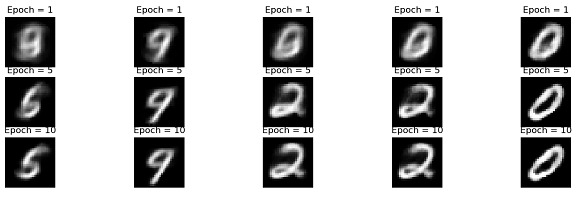
此代码绘制训练好的自编码器模型的原始图像和重建图像。变量outputs包含有关模型输出的数据,例如重建图像和在不同训练 epoch 中记录的损失值。使用list_epochs变量来绘制特定 epoch 的重建图像。
该程序绘制给定 epoch 的最后一批中的前五张重建图像。
示例
# Plot the re-constructed images
# Initializing the counter
count = 1
# Plotting the reconstructed images
list_epochs = [1, 5, 10]

# Iterate over specified epochs
for val in list_epochs:

   # Extract recorded information
   temp = outputs[val]['out'].detach().numpy()
   title_text = f"Epoch = {val}"

   # Plot first 5 images of the last batch
   for idx in range(5):
      plt.subplot(7, 5, count)
      plt.title(title_text)
      plt.imshow(temp[idx].reshape(28,28), cmap= 'gray')
      plt.axis('off')

      # Increment the count
      count+=1

# Plot of the original images

# Iterating over first five
# images of the last batch
for idx in range(5):

   # Obtaining image from the dictionary
   val = outputs[10]['img']

   # Plotting image
   plt.subplot(7,5,count)
   plt.imshow(val[idx].reshape(28, 28),
               cmap = 'gray')
   plt.title("Original Image")
   plt.axis('off')

   # Increment the count
   count+=1

plt.tight_layout()
plt.show()
输出
步骤5:测试集性能评估
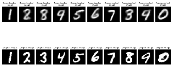
此代码是关于如何在测试集上评估训练好的自编码器模型的性能的示例。
代码根据对重建图像的视觉检查得出结论,自编码器模型在测试集上表现良好。如果模型在测试集上表现良好,则它很可能在新数据上表现良好。
示例
outputs = {}

# Extract the last batch dataset
img, _ = list(test_loader)[-1]

img = img.reshape(-1, 28 * 28)

#Generating output
out = model(img)

# Storing results in the dictionary
outputs['img'] = img
outputs['out'] = out

# Initialize subplot count
count = 1
val = outputs['out'].detach().numpy()

# Plot first 10 images of the batch
for idx in range(10):
   plt.subplot(2, 10, count)
   plt.title("Reconstructed \n image")
   plt.imshow(val[idx].reshape(28, 28), cmap='gray')
   plt.axis('off')

   # Increment subplot count
   count += 1
# Plotting original images
# Plotting first 10 images
for idx in range(10):
   val = outputs['img']
   plt.subplot(2, 10, count)
   plt.imshow(val[idx].reshape(28, 28), cmap='gray')
   plt.title("Original Image")
   plt.axis('off')
   count += 1

plt.tight_layout()
plt.show()
输出
结论
总之,自编码器是强大的神经网络,可以应用于许多不同的任务,包括数据压缩、异常检测和图像生成。TensorFlow、Keras和PyTorch是一些使自编码器开发简单的Python工具。通过理解架构和调整参数,可以构建非常强大的自编码器模型。随着机器学习领域的进步,自编码器很可能继续成为各种应用的有用工具。

浏览量:585
