
 数据结构
数据结构 网络
网络 关系型数据库管理系统 (RDBMS)
 操作系统
操作系统 Java
Java iOS
iOS HTML
HTML CSS
CSS Android
 Python
 C语言编程
C语言编程 C++
C++ C#
C# MongoDB
 MySQL
MySQL Javascript
 PHP
PHP使用Python进行机器学习的医疗保险价格预测
与许多其他领域一样,预测分析在金融和保险领域也相当有用。使用这种机器学习技术,我们可以找出有关任何保险单的有用信息,从而节省大量资金。在这里,我们将对医疗保险数据集使用这种预测分析方法。
这里的问题陈述是,我们拥有一些具有某些属性的人的数据集。使用Python中的机器学习,我们必须从这个数据集中找出相关信息,并且还必须预测一个人将不得不支付的保险价格。
算法
步骤 1 − 导入numpy、pandas、matplotlib、seaborn和sklearn等库,并将数据集加载为pandas数据帧。
步骤 2 − 为了清理数据,首先检查空值。如果发现空值,则查找各种特征之间的关系并估算空值。如果没有,那么我们就可以开始了。
步骤 3 − 现在执行EDA,这意味着检查各种自变量之间的关系。
步骤 4 − 查找异常值并调整它们。
步骤 5 − 绘制热图以找出高度相关的变量。
步骤 6 − 将数据集拆分为测试集和训练集,并使用StandardScaler标准化数据。
步骤 7 − 现在在这个数据上训练一些机器学习模型,并使用mape来检查哪个模型效果最好。
示例
在这个例子中,我们将使用一个医疗保险数据集(你可以在此处找到),然后我们将执行预测一个人必须为特定医疗保险支付的保险价格所需的各种步骤。
#import the required libraries
import numpy as np
import pandas as pd
import seaborn as sb
import matplotlib.pyplot as plt
from sklearn.model_selection import train_test_split
from sklearn.preprocessing import StandardScaler, LabelEncoder
from sklearn.metrics import mean_absolute_percentage_error as mape
from sklearn.linear_model import LinearRegression, Lasso, Ridge
from xgboost import XGBRegressor
from sklearn.ensemble import RandomForestRegressor, AdaBoostRegressor
import warnings
warnings.filterwarnings('ignore')
#load and print the dataset
df = pd.read_csv('insurance_dataset.csv')
df.head()
df.shape
df.info()
df.describe()
#check for null values
df.isnull().sum()
#see the relation between independent features
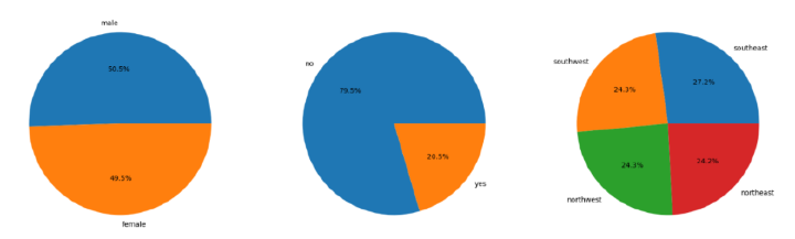
#pie charts
features = ['sex', 'smoker', 'region']
plt.subplots(figsize=(20, 10))
for i, col in enumerate(features):
plt.subplot(1, 3, i + 1)
x = df[col].value_counts()
plt.pie(x.values, labels=x.index, autopct='%1.1f%%')
plt.show()
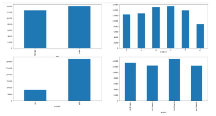
#bar graphs
features = ['sex', 'children', 'smoker', 'region']
plt.subplots(figsize=(20, 10))
for i, col in enumerate(features):
plt.subplot(2, 2, i + 1)
df.groupby(col).mean()['charges'].plot.bar()
plt.show()
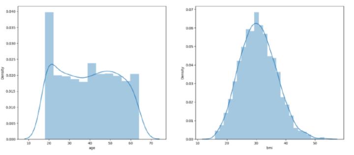
#plots
features = ['age', 'bmi']
plt.subplots(figsize=(17, 7))
for i, col in enumerate(features):
plt.subplot(1, 2, i + 1)
sb.distplot(df[col])
plt.show()
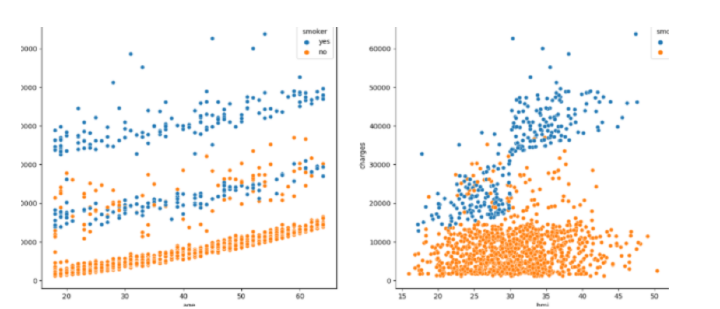
#scatterplots
features = ['age', 'bmi']
plt.subplots(figsize=(17, 7))
for i, col in enumerate(features):
plt.subplot(1, 2, i + 1)
sb.scatterplot(data=df, x=col, y='charges', hue='smoker')
plt.show()
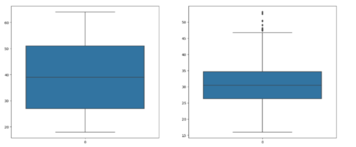
#check for outliers
features = ['age', 'bmi']
plt.subplots(figsize=(17, 7))
for i, col in enumerate(features):
plt.subplot(1, 2, i + 1)
sb.boxplot(df[col])
plt.show()
#adjust the outliers
df.shape, df[df['bmi']<45].shape
df = df[df['bmi']<50]
for col in df.columns:
if df[col].dtype == object:
le = LabelEncoder()
df[col] = le.fit_transform(df[col])
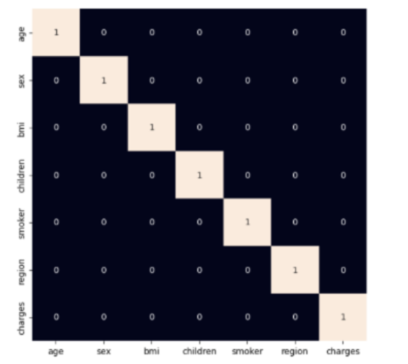
#use heatmap to see highly correlated variables
plt.figure(figsize=(7, 7))
sb.heatmap(df.corr() > 0.8, annot=True, cbar=False)
plt.show()
#split the dataset into train and test sets
features = df.drop(['charges'], axis=1)
target = df['charges']
X_train, X_val,\
Y_train, Y_val = train_test_split(features, target, test_size=0.1, random_state=22)
X_train.shape, X_val.shape
#fit the data
scaler = StandardScaler()
X_train = scaler.fit_transform(X_train)
X_val = scaler.transform(X_val)
#find the performance of various models
models = [LinearRegression(), XGBRegressor(),
RandomForestRegressor(), AdaBoostRegressor(),
Lasso(), Ridge()]
for i in range(6):
models[i].fit(X_train, Y_train)
print(f'{models[i]} : ')
pred_train = models[i].predict(X_train)
print('Training Error : ', mape(Y_train, pred_train))
pred_val = models[i].predict(X_val)
print('Validation Error : ', mape(Y_val, pred_val))
print()
导入所需的库后,数据集将存储到python数据框中。然后,代码检查数据集中是否存在空值,并相应地绘制饼图和条形图以可视化数据集中性别、地区和吸烟者列的分布和比例。
然后,显示直方图和散点图以可视化年龄和bmi与费用变量的分布和关系。检查年龄和bmi列,并通过过滤掉极值来进行修改。之后,将性别、吸烟者和地区列中的值转换为数值形式,并创建一个热图以可视化数据集中列之间的关系。
然后将数据集拆分为训练集和验证集。根据训练集和验证集上的平均绝对百分比误差,训练和评估各种回归模型。
输出
<class 'pandas.core.frame.DataFrame'>
RangeIndex: 1338 entries, 0 to 1337
Data columns (total 7 columns):
 #   Column    Non-Null Count  Dtype
---  ------    --------------  -----
 0   age       1338 non-null   int64
 1   sex       1338 non-null   object
 2   bmi       1338 non-null   float64
 3   children  1338 non-null   int64
 4   smoker    1338 non-null   object
 5   region    1338 non-null   object
 6   charges   1338 non-null   float64
dtypes: float64(2), int64(2), object(3)
memory usage: 73.3+ KB
LinearRegression() −
Training Error :  0.42160312973300035
Validation Error :  0.36819643775368394
XGBRegressor() −
Training Error :  0.07414118093426757
Validation Error :  0.43487251393507226
RandomForestRegressor() −
Training Error :  0.11931475932482996
Validation Error :  0.33574049059141486
AdaBoostRegressor() −
Training Error :  0.6166709629183661
Validation Error :  0.5758503954769271
Lasso() −
Training Error :  0.42160217445355996
Validation Error :  0.36821456297631355
Ridge() −
Training Error :  0.42182509871430085
Validation Error :  0.3685041955294438
您可以看到XGBRegressor的MAPE(平均绝对百分比误差)值最小。这意味着该模型预测的价格非常接近实际价格,因此可以认为是该项目的最佳模型。
结论
为了进行这种医疗保险价格预测,您还可以使用其他模型,例如K近邻(KNN)、支持向量机(SVM)、随机森林(RF)和朴素贝叶斯等。此外,此处的数据大多已预处理。但是,您可以根据需要自行预处理它。此外,可以以相同的方式对具有其他几个特征的数据集进行类似的预测。

515 次浏览
