
 数据结构
数据结构 网络
网络 关系数据库管理系统 (RDBMS)
 操作系统
操作系统 Java
Java iOS
iOS HTML
HTML CSS
CSS Android
 Python
 C语言编程
C语言编程 C++
C++ C#
C# MongoDB
 MySQL
MySQL Javascript
 PHP
PHPPython 实现数字带通巴特沃斯滤波器
带通滤波器是一种只允许特定频率范围内的信号通过,而阻挡其他频率范围外信号的滤波器。巴特沃斯带通滤波器的设计目标是使其在通带内的频率响应尽可能平坦。以下是数字带通巴特沃斯滤波器的规格说明。
滤波器的采样率约为 40 kHz。
通带截止频率范围为 1400 Hz 到 2100 Hz。
阻带截止频率范围为 1050 Hz 到 2450 Hz。
通带纹波为 0.4 分贝。
阻带最小衰减为 50 分贝。
实现数字带通巴特沃斯滤波器
实现数字带通巴特沃斯滤波器是一个循序渐进的过程。让我们详细了解每个步骤。
步骤 1 − 首先,我们需要定义输入信号的采样频率 fs、下限截止频率 f1、上限截止频率 f2 和滤波器的阶数。如果我们确定了较高的滤波器阶数,则会导致更陡峭的滚降,从而造成相位失真。
步骤 2 − 接下来,我们需要使用下面的公式计算下限和上限截止频率 f1 和 f2 的归一化频率 wn1 和 wn2。
$\mathrm{wn = 2 * fn / fs}$
步骤 3 − 之后,我们可以使用 scipy.signal.butter() 函数设计指定阶数和归一化频率的巴特沃斯滤波器,并将 btype 参数指定为 band。
步骤 4 − 现在,我们将使用 scipy.signal.filtfilt() 函数对给定的输入信号应用滤波器,以执行零相位滤波。
示例
在下面的示例中,我们使用上述步骤实现数字带通巴特沃斯滤波器。
import numpy as np
import matplotlib.pyplot as plt
from scipy.signal import butter, filtfilt
def butter_bandpass(lowcut, highcut, fs, order=5):
nyq = 0.5 * fs
low = lowcut / nyq
high = highcut / nyq
b, a = butter(order, [low, high], btype='band')
return b, a
def butter_bandpass_filter(data, lowcut, highcut, fs, order=5):
b, a = butter_bandpass(lowcut, highcut, fs, order=order)
y = filtfilt(b, a, data)
return y
fs = 1000
t = np.arange(0, 1, 1/fs)
f1 = 10
f2 = 50
sig = np.sin(2*np.pi*f1*t) + np.sin(2*np.pi*f2*t)
order = 4
filtered = butter_bandpass_filter(sig, f1, f2, fs, order)
print("The length of frequencies:",len(filtered))
print("The Butterworth bandpass filter output of first 50 frequencies:",filtered[:50])
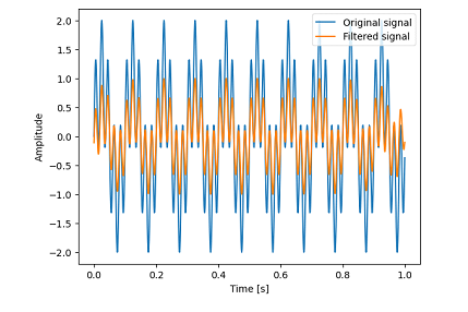
fig, ax = plt.subplots()
ax.plot(t, sig, label='Original signal')
ax.plot(t, filtered, label='Filtered signal')
ax.set_xlabel('Time [s]')
ax.set_ylabel('Amplitude')
ax.legend()
plt.show()
输出
The length of frequencies: 1000
The Butterworth bandpass filter output of first 50 frequencies: [-0.11133763  0.06408296  0.22202113  0.34937958  0.4360314   0.47578308
  0.46696733  0.41260559  0.32012087  0.20062592  0.06785282 -0.0631744
 -0.17759655 -0.26216511 -0.30653645 -0.30428837 -0.2535591  -0.15724548
 -0.02273955  0.13877185  0.31337781  0.48578084  0.64077163  0.76469778
  0.84678346  0.88017133  0.86258464  0.79654483  0.68912261  0.55124662
  0.39663647  0.24046415  0.09787411 -0.01749368 -0.0948334  -0.12722603
 -0.11231195 -0.05251783  0.04518472  0.16996505  0.30819725  0.44479774
  0.5647061   0.65436437  0.70305015  0.70393321  0.65475213  0.5580448
  0.42091007  0.25432388]

更新于: 2023-10-31
浏览量 1K+

广告