
 数据结构
数据结构 网络
网络 关系数据库管理系统 (RDBMS)
 操作系统
操作系统 Java
Java iOS
iOS HTML
HTML CSS
CSS Android
 Python
 C语言编程
C语言编程 C++
C++ C#
C# MongoDB
 MySQL
MySQL Javascript
 PHP
PHP如何在Python中绘制带有滚动平均线的时序图?
在这篇文章中,我们将介绍两种使用Python绘制带有滚动平均线的时序图的方法。这两种方法都使用了像Matplotlib、Pandas和Seaborn这样知名的库,这些库提供了强大的数据处理和可视化功能。按照这些方法,您可以高效地可视化带有滚动平均线的时序数据,并了解其总体行为。
这两种方法都使用了类似的步骤序列,包括加载数据,将日期列转换为DateTime对象,计算滚动平均值以及生成图表。主要区别在于用于生成图表的库和函数。您可以自由选择最适合您的知识和偏好的方法。
方法
使用Pandas和Matplotlib。
使用Seaborn和Pandas。
注意:此处使用的数据如下所示:
文件名可以根据需要更改。这里文件名是dataS.csv。
date,value
2022-01-01,10
2022-01-02,15
2022-01-03,12
2022-01-04,18
2022-01-05,20
2022-01-06,17
2022-01-07,14
2022-01-08,16
2022-01-09,19
让我们检查一下这两种方法:
方法1:使用Pandas和Matplotlib
此方法使用Pandas和matplotlib库来绘制时序图。流行的绘图库Matplotlib提供了丰富的工具,用于创建静态、动画和交互式可视化。另一方面,强大的数据处理库Pandas提供了有用的数据结构和函数,用于处理结构化数据,包括时间序列。
算法
步骤1 - 导入用于数据可视化的matplotlib.pyplot以及用于数据处理的pandas。
步骤2 - 使用pd.read_csv()从CSV文件加载时间序列数据。假设文件名为'dataS.csv'。
步骤3 - 使用pd.to_datetime()将DataFrame的'date'列转换为DateTime对象。
步骤4 - 使用data.set_index('date', inplace=True)将'date'列设置为DataFrame的索引。
步骤5 - 指定滚动平均值计算的窗口大小。根据预期的窗口大小调整window_size变量。
步骤6 - 使用data['value'].rolling(window=window_size).mean()计算'value'列的滚动平均值。
步骤7 - 使用plt.figure()创建图表。使用figsize=(10, 6)根据需要调整图表大小。
步骤8 - 使用plt.plot(data.index, data['value'], label='Actual')绘制实际值。
步骤9 - 使用plt.plot(data.index, rolling_avg, label='Rolling Average')绘制滚动平均值。
步骤10 - 使用plt.xlabel()和plt.ylabel()设置x轴和y轴的标签。
步骤11 - 使用plt.title()设置图表的标题。
步骤12 - 使用plt.legend()显示已绘制线的图例。
步骤13 - 使用plt.grid(True)在图表上启用网格。
步骤14 - 使用plt.show()显示图表。
程序
#pandas library is imported
import pandas as pd
import matplotlib.pyplot as plt
# Load the time series data
data = pd.read_csv('dataS.csv')
# Transform the column date to a datetime object
data['date'] = pd.to_datetime(data['date'])
# Put the column date column as the index
data.set_index('date', inplace=True)
# Calculate the rolling average
window_size = 7 # Adjust the window size as per your requirement
rolling_avg = data['value'].rolling(window=window_size).mean()
# Create the plot
plt.figure(figsize=(10, 6)) # Adjust the figure size as needed
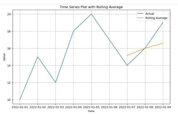
plt.plot(data.index, data['value'], label='Actual')
plt.plot(data.index, rolling_avg, label='Rolling Average')
plt.xlabel('Date')
plt.ylabel('Value')
plt.title('Time Series Plot with Rolling Average')
plt.legend()
plt.grid(True)
plt.show()
输出
方法2:使用Seaborn和Pandas
这介绍了Seaborn的使用,Seaborn是一个基于Matplotlib的高级数据可视化框架。Seaborn是创建视觉上吸引人的时间序列图的一个很好的选择,因为它提供了一个简单而有吸引力的统计图形界面。
步骤1 - 导入seaborn、pandas和matplotlib.pyplot库。
步骤2 - 使用pd.read_csv()函数从'dataS.csv'文件加载时间序列数据,并将其存储在data变量中。
步骤3 - 使用pd.to_datetime()函数将data DataFrame中的'date'列转换为datetime对象。
步骤4 - 使用set_index()方法将'date'列设置为DataFrame的索引。
步骤5 - 指定滚动平均值计算的窗口大小。根据需要调整window_size变量。
步骤6 - 使用data DataFrame的'value'列上的rolling()函数并指定窗口大小来计算滚动平均值。
步骤7 - 使用plt.figure(figsize=(10, 6))创建一个具有特定大小的新图表。
步骤8 - 使用sns.lineplot()和data DataFrame的'value'列绘制实际时间序列数据。
步骤9 - 使用sns.lineplot()和rolling_avg变量绘制滚动平均值。
步骤10 - 使用plt.xlabel()设置x轴标签。
步骤11 - 使用plt.ylabel()设置y轴标签。
步骤12 - 使用plt.title()设置图表的标题。
步骤13 - 使用plt.legend()显示图例。
步骤14 - 使用plt.grid(True)在图表上添加网格线。
步骤15 - 使用plt.show()显示图表。
示例
import pandas as pd
import seaborn as sns
import matplotlib.pyplot as plt
# Step 1: Fill the time series data with the csv file provided
data = pd.read_csv('your_data.csv')
# Transform the column date to the object of DateTime
data['date'] = pd.to_datetime(data['date'])
# Put the column data as the index
data.set_index('date', inplace=True)
# Adjust the window size as per your requirement
# and then compute the rolling average
window_size = 7
# rolling_avg = data['value'].rolling(window=window_size).mean()
# Build the plot utilizing Seaborn
plt.figure(figsize=(10, 6))
# Adjust the figure size as needed
sns.lineplot(data=data['value'], label='Actual')
sns.lineplot(data=rolling_avg, label='Rolling Average')
plt.xlabel('Date')
plt.ylabel('Value')
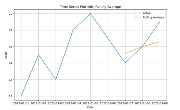
plt.title('Time Series Plot with Rolling Average')
plt.legend()
plt.grid(True)
plt.show()
输出
结论
通过使用像Pandas和Matplotlib这样的Python模块,可以轻松创建滚动平均时间序列图。这些可视化效果使我们能够成功地分析时间相关数据中的趋势和模式。清晰的代码概述了如何导入数据、转换日期列、计算滚动平均值以及可视化结果。这些方法使我们能够理解数据的行为并做出明智的结论。金融、经济学和气候研究都将时间序列分析和可视化作为有效的工具。

896 次浏览
