用Python实现雅可比方法求解线性方程组

---

这是解决如下所示线性方程组最直接的迭代方法。

$$\mathrm{a_{1,1}\: x_{1} \: + \: a_{1,2} \: x_{2} \: + \: \dotso\dotso \: + \: a_{1,n} \: x_{n} \: = \: b_{1}}$$

$$\mathrm{a_{2,1} \: x_{1} \: + \: a_{2,2} \: x_{2} \: + \: \dotso\dotso \: + \: a_{2,n} \: x_{n} \: = \: b_{2}}$$

$$\mathrm{\vdots}$$

$$\mathrm{a_{n,1} \: x_{1} \: + \: a_{n,2} \: x_{2} \: + \: \dotso\dotso \: + \: a_{n,n} \: x_{n} \: = \: b_{n}}$$

基本思想是：将每个线性方程重新排列，将一个新的变量移到左边。然后，从对每个变量的初始猜测开始确定新值。在接下来的迭代中，新值将用作更准确的猜测。重复此迭代过程，直到满足每个变量的收敛条件，从而得到最终收敛的答案。

雅可比算法

雅可比算法如下：

• 从未知数（x）的一些初始猜测数组开始。

• 通过在如下所示的方程重新排列形式中代入x的猜测值来计算新的x：

$$\mathrm{x_{i_{new}} \: = \: − \frac{1}{a_{i,i}}(\sum_{j=1,j \neq i}^n a_{i,j}x_{j_{guess}} \: − \: b_{i})}$$

现在，$\mathrm{x_{i_{new}}}$将是当前迭代中获得的新x值。

• 下一步是评估新值和猜测值之间的误差，即$\mathrm{\lvert x_{new} \: − \: x_{guess} \rvert}$。如果误差大于某个收敛准则（我们将其设为$\mathrm{10^{−5}}$），则将新值赋给旧猜测值，即$\mathrm{x_{guess} \: = \: x_{new}}$，然后开始下一次迭代。

• 否则，$\mathrm{x_{new}}$是最终答案。

雅可比算法——示例

让我们通过以下示例来演示该算法：

$$\mathrm{20x \: + \: y \: − \: 2z \: = \: 17}$$

$$\mathrm{3x \: + \: 20y \: − \: z \: = \: −18}$$

$$\mathrm{2x \: − \: 3y \: + \: 20z \: = \: 25}$$

将上述方程重新排列如下：

$$\mathrm{x_{new} \: = \: (−y_{guess} \: + \: 2z_{guess} \: + \: 17)/20}$$

$$\mathrm{y_{new} \: = \: (−3x_{guess} \: + \: z_{guess} \: − \: 18)/20}$$

$$\mathrm{z_{new} \: = \: (−2x_{guess} \: + \: 3y_{guess} \: + \: 25)/20}$$

现在，这些方程将在while循环中求解，以根据猜测值获得未知数的新值。

实现雅可比方法的Python程序

下面显示了实现雅可比方法（按方程实现）的程序：

示例

# Importing module for plotting and array
from pylab import *
from numpy import *

# Initial guess to start with
xg=0
yg=0
zg=0

# Setting error to move into the while loop
error=1

# Setting up iteration counter
count=0

while error>1.E-5:
   count+=1
    
   #Evaluating new values based on old guess
   x=(17-yg+2*zg)/20
   y=(zg-18-3*xg)/20
   z=(25-2*xg+3*yg)/20

   # Error evaluation and plotting
   error = abs(x-xg)+abs(y-yg)+abs(z-zg)
   figure(1,dpi=300)
   semilogy(count,error,'ko')
   xlabel('iterations')
   ylabel('error')

   # Updating the Guess for next iteration.
   xg=x
   yg=y
   zg=z

savefig('error_jacobi.jpg')
print(f'x={round(x,5)}, y={round(y,5)}, z={round(z,5)}')

输出

程序输出将是

$$\mathrm{x \: = \: 1.0 \: , \: y \: = \: −1.0 \: , \: z \: = \: 1.0}$$

下图显示了每次迭代次数的误差变化：

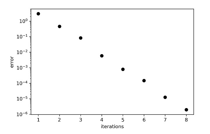
可以观察到，收敛解在第8次迭代时达到。

但是，我认为如果我们可以将线性方程组的元素输入到矩阵中并以矩阵形式而不是方程形式求解它们，将会更好。因此，执行此任务的过程代码如下：

示例

# Importing module
from pylab import *
from numpy import *

#-----------------------------------------#
# Array of coefficients of x
a=array([[20,1,-2],[3,20,-1],[2,-3,20]])

# Array of RHS vector
b=array([17,-18,25])

# Number of rows and columns
n=len(b)
#-----------------------------------------#


# Setting up the initial guess array
xg=zeros(len(b))

# Starting error to enter in loop
error=1

# Setting iteration counter
count=0

# Generating array for new x
xn=empty(len(b)) 
#-----------------------------------------#


while error>1.E-5:
   count+=1
   for i in range(n):
      sum1=0
      for j in range(n):
         if i!=j:
            sum1=sum1+a[i,j]*xg[j]
      xn[i]=(-1/a[i,i])*(sum1-b[i])


   # Error evaluation and plotting
   error = sum(abs(xn-xg))
    
   figure(1,dpi=300)
   semilogy(count,error,'ko')
   xlabel('iterations')
   ylabel('error')

   # Substituting new value as the Guess for next iteration
   xg=xn.copy()
#-----------------------------------------#

savefig('error_jacobi.jpg')
print('x: ',xn)

输出

x: [ 1.00000007 -0.99999983 1.00000005]

结论

在本教程中，我们解释了如何使用Python来模拟雅可比迭代法求解联立线性方程组。讨论了两种方法：方程法和矩阵法。