XGBoost - 自举法

自举法可以与可替换抽样相结合，对数据进行重采样并生成许多训练集。因此，XGBoost 中的自举策略可以定义为一种方法，在这种方法中，我们在数据的许多随机子集上训练模型以改进它。

它是如何工作的？

为每个重采样集训练一个 XGBoost 模型，并对测试数据点生成预测。这些预测的分布提供了对预测不确定性的粗略估计。

因此，XGBoost 中的自举策略指的是通过在数据的许多随机子集上训练模型来改进模型的一种方法。

XGBoost 生成大量的小模型，每个模型都在可用数据的一部分上进行训练。这种随机抽样称为“自举”。XGBoost 组合这些小模型的输出，并在数据的各种子集上进行训练，以生成单个强大的预测。

通过使用不同的随机样本，此策略试图减少错误并提高模型准确性。它还有助于 XGBoost 模型避免过拟合，过拟合是指模型在训练数据上表现良好但在新数据上表现不佳的情况。

这类似于人们通过获得新经验来学习的方式。

将自举法应用于模型

正如我们在自举法中所看到的，使用训练数据的重采样版本训练多个模型，并将其预测结果结合起来。基本思想是随机选择数据，自举多个模型，然后对以前从未见过的测试数据进行预测。通过平均预测并计算其可变性，我们可以生成置信区间，显示预测中不确定性的程度。

因此，让我们看看将自举法应用于 XGBoost 模型的步骤 -

1. 导入必要的库并生成合成数据

首先，我们将加载 XGBoost、NumPy 和 Matplotlib 等库来训练和分析模型。接下来，我们生成合成数据来训练模型。

# Importing libraries here
import xgboost as xgb  
import numpy as np  
import matplotlib.pyplot as plt

# Generate random training and testing data
np.random.seed(123)  
X_train_data = np.random.rand(150, 8)  
y_train_target = np.random.rand(150)  

# Generate 30 samples with 8 features for testing
X_test_data = np.random.rand(30, 8)

2. 自举

现在，我们将使用上述自举法创建多个模型。每次我们随机对训练集进行重采样，将 XGBoost 模型拟合到它，然后对测试集进行预测。当我们试图获取从多个自举数据集收集的预测集合时，此方法将重复多次。

# Number of bootstrapped models
n_iterations = 120  
# List to store predictions from each model
all_preds = []  

for iteration in range(n_iterations):
    # Create a bootstrapped dataset 
    sampled_indices = np.random.choice(len(X_train_data), len(X_train_data), replace=True)
    X_resampled_data, y_resampled_target = X_train_data[sampled_indices], y_train_target[sampled_indices]
    
    # Initialize and train an XGBoost regression model
    xgboost_model = xgb.XGBRegressor()
    xgboost_model.fit(X_resampled_data, y_resampled_target)
    
    # Make predictions on the test data
    test_predictions = xgboost_model.predict(X_test_data)
    all_preds.append(test_predictions)

# Convert the list of predictions to a NumPy array
all_preds = np.array(all_preds)

# Calculate the mean and standard deviation 
avg_preds = np.mean(all_preds, axis=0)
std_dev_preds = np.std(all_preds, axis=0)

# Calculate 95% confidence intervals 
lower_confidence_bound = avg_preds - 1.96 * std_dev_preds
upper_confidence_bound = avg_preds + 1.96 * std_dev_preds

可视化结果

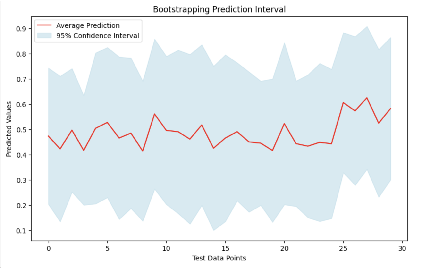
通过取所有预测的平均值（均值）及其标准差，我们可以创建一个预测区间。这将帮助我们了解实际数据可能落入的范围，并提供预测不确定性的度量。我们可以通过绘制平均预测并突出显示其周围的置信区间来查看结果。

# Visualization of the predictions with confidence intervals
# Set the figure size
plt.figure(figsize=(10, 6))  

# Plot the mean predictions
plt.plot(avg_preds, label='Average Prediction', color='red')

# Fill the area between the lower and upper confidence bounds
plt.fill_between(range(len(avg_preds)), lower_confidence_bound, upper_confidence_bound, color='lightblue', alpha=0.5, label='95% Confidence Interval')

# Add title and labels to the plot
plt.title('Bootstrapping Prediction Interval') 
plt.xlabel('Test Data Points')  
plt.ylabel('Predicted Values')  

# Add a legend to describe the plot lines
plt.legend()  
# Display the plot
plt.show()

输出

这将产生以下结果 -

打印页面