使用 Python 在统计学中展示 Nakagami 分布

---

在给定的问题陈述中，我们必须创建一个算法，以借助 Python 及其库来展示统计学中的 Nakagami 分布。因此，在本文中，我们将使用 Python 的 matplotlib、numpy 和 scipy 库来解决给定的问题。

什么是统计学中的 Nakagami 分布？

Nakagami 分布基本上是一个概率分布。它包含参数、样本数据集和概率分布的模型描述。此分布主要用于通信中，以模拟通过多个路径到达接收器的信号。

理解问题的逻辑

手头的问题是使用 Python 及其库来展示 Nakagami 分布。因此，我们将首先导入所有必要的库，导入后，我们将生成一个数据集，在此数据集上我们将创建 Nakagami 分布。然后，我们将计算概率密度函数，然后借助绘图方法绘制分布图。

算法

• 步骤 1 - 首先，我们将导入必要的库

from scipy.stats import nakagami
import numpy as nmp
import matplotlib.pyplot as pplt

• 步骤 2 - 然后我们将生成 x 的值

x = nmp.linspace(0, 8, 200)

• 步骤 3 - 下一步是定义 Nakagami 分布的参数

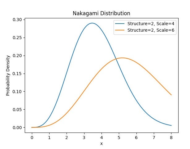
structure1, scale1 = 2, 4
structure2, scale2 = 2, 6

• 步骤 4 - 声明参数后，我们需要为每个参数计算概率密度函数（也称为 PDF 值）。在这里，我们将使用 Nakagami 的 pdf 函数来计算概率密度函数，并在其中传递参数的值。

prob_den_fun1 = nakagami.pdf(x, structure1, scale=scale1)
prob_den_fun2 = nakagami.pdf(x, structure2, scale=scale2)

• 步骤 5 - 现在，我们将借助 matplotlib 库的绘图函数绘制概率密度函数。

pplt.plot(x, prob_den_fun1, label='Structure={}, Scale={}'.format(structure1, scale1))
pplt.plot(x, prob_den_fun2, label='Structure={}, Scale={}'.format(structure2, scale2))

• 步骤 6 - 绘制 PDF 后，我们将向绘图添加标签，并使用 matplotlib 的 legend 函数来描述图形中的项目。

pplt.xlabel('x')
pplt.ylabel('Probability Density')
pplt.title('Nakagami Distribution')
pplt.legend()

• 步骤 7 - 最后，我们将使用 matplotlib 的 show 方法显示我们创建的绘图。

pplt.show()

示例

from scipy.stats import nakagami
import numpy as nmp
import matplotlib.pyplot as pplt

x = nmp.linspace(0, 8, 200)

structure1, scale1 = 2, 4
structure2, scale2 = 2, 6

prob_den_fun1 = nakagami.pdf(x, structure1, scale=scale1)
prob_den_fun2 = nakagami.pdf(x, structure2, scale=scale2)

pplt.plot(x, prob_den_fun1, label='Structure={}, Scale={}'.format(structure1, scale1))
pplt.plot(x, prob_den_fun2, label='Structure={}, Scale={}'.format(structure2, scale2))

pplt.xlabel('x')
pplt.ylabel('Probability Density')
pplt.title('Nakagami Distribution')
pplt.legend()
pplt.show()

输出

结论

正如我们已经成功创建了代码来演示 scipy.stats、matplotlib 和 numpy 模块的使用，以使用不同参数集的概率密度函数或 PDF 来展示 Nakagami 分布。我们提供了简单高效的代码，具有 O(1) 的时间复杂度。在我们的代码中，我们可以根据需要调整参数并优化 Nakagami 分布，并且我们可以看到它如何反映形状和曲线。总的来说，该代码提供了一个简单有效的方法来展示 Nakagami 分布。