SciPy - integrate.romb() 方法

SciPy integrate.romb() 方法用于执行数值积分或罗姆伯格积分任务。此方法还帮助我们根据样本/坐标点绘制图形。

语法

以下为 SciPy integrate.romb() 方法的语法 -

romb(y, dx = int_val/float_val/1.0)

参数

此函数接受以下参数 -

• y: 此参数确定离散点上的数组函数，并且这些点被认为是均匀间隔开的。
• dx: 此参数确定点之间的间隔，如果未指定，其默认值为 1.0。

返回值

此方法返回类型为浮点数的估计值。

示例 1

以下为展示简单的积分函数 SciPy integrate.romb() 方法，即 f(x) = x²，其中积分区间在 0 到 1 之间。最终值基于五个离散点。

import numpy as np
from scipy import integrate

# define the function values at discrete points
x = np.linspace(0, 1, 5)
y = x**2 

# calculate the integral
res_integral = integrate.romb(y, dx=x[1] - x[0])

# display the result
print(res_integral)

输出

以上代码产生以下结果 -

0.3333333333333333

示例 2

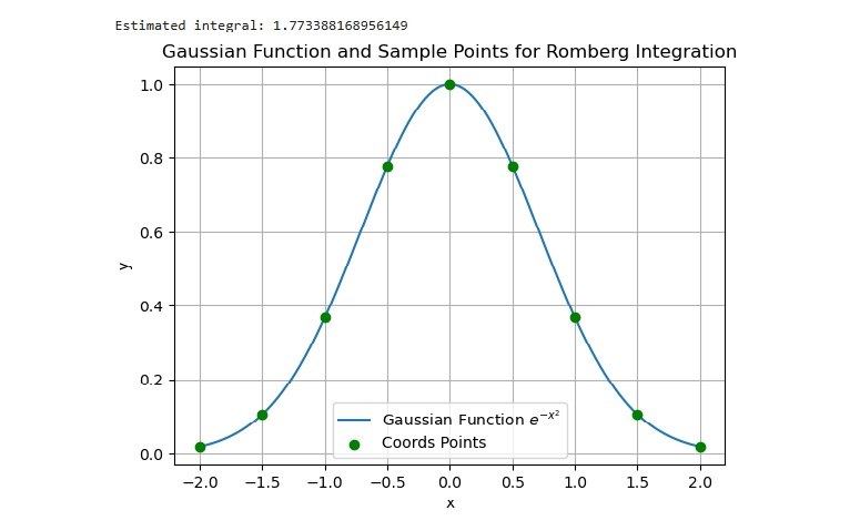
这个程序演示了高斯函数（即 e^-x2）在 -2 到 2 之间区间的数值积分，并且该函数值被表示为九个点（x 轴）。

import numpy as np
from scipy.integrate import romb
import matplotlib.pyplot as plt

# define the function values at discrete points
x = np.linspace(-2, 2, 9)
y = np.exp(-x**2)

# calculate the integral
res_integral = romb(y, dx=x[1] - x[0])

# display the result
print(f"Estimated integral: {res_integral}")

# plot the Gaussian function and the points used in Romberg integration
x_fine = np.linspace(-2, 2, 1000)
y_fine = np.exp(-x_fine**2)

plt.plot(x_fine, y_fine, label='Gaussian Function $e^{-x^2}$')
plt.scatter(x, y, color='green', zorder=5, label='coords Points')

plt.title('Gaussian Function and Sample Points for Romberg Integration')
plt.xlabel('x')
plt.ylabel('y')
plt.legend()
plt.grid(True)
plt.show()

输出

以上代码产生以下结果 -