机器学习 - 多项式回归

多项式线性回归是一种回归分析，其中自变量和因变量之间的关系被建模为n次多项式函数。与简单和多元线性回归中的线性关系相比，多项式回归允许捕获变量之间更复杂的关系。

Python 实现

以下是用 Scikit-Learn 中的波士顿房价数据集实现多项式线性回归的示例：

示例

from sklearn.datasets import load_boston
from sklearn.model_selection import train_test_split
from sklearn.linear_model import LinearRegression
from sklearn.preprocessing import PolynomialFeatures
from sklearn.metrics import mean_squared_error, r2_score
import numpy as np
import matplotlib.pyplot as plt

# Load the Boston Housing dataset
boston = load_boston()

# Split the dataset into training and testing sets
X_train, X_test, y_train, y_test = train_test_split(boston.data,
boston.target, test_size=0.2, random_state=0)

# Create a polynomial features object with degree 2
poly = PolynomialFeatures(degree=2)

# Transform the input data to include polynomial features
X_train_poly = poly.fit_transform(X_train)
X_test_poly = poly.transform(X_test)

# Create a linear regression object
lr_model = LinearRegression()

# Fit the model on the training data
lr_model.fit(X_train_poly, y_train)

# Make predictions on the test data
y_pred = lr_model.predict(X_test_poly)

# Calculate the mean squared error
mse = mean_squared_error(y_test, y_pred)

# Calculate the coefficient of determination
r2 = r2_score(y_test, y_pred)

print('Mean Squared Error:', mse)
print('Coefficient of Determination:', r2)

# Sort the test data by the target variable
sort_idx = X_test[:, 12].argsort()

X_test_sorted = X_test[sort_idx]
y_test_sorted = y_test[sort_idx]

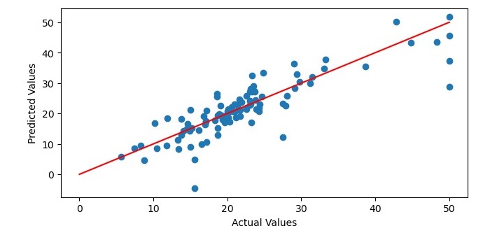
# Plot the predicted values against the actual values
plt.figure(figsize=(7.5, 3.5))
plt.scatter(y_test_sorted, y_pred[sort_idx])
plt.xlabel('Actual Values')
plt.ylabel('Predicted Values')

# Add a regression line to the plot
x = np.linspace(0, 50, 100)
y = x
plt.plot(x, y, color='red')

# Show the plot
plt.show()

输出

执行程序时，它将生成以下图表作为输出，并在终端上打印均方误差和决定系数：

Mean Squared Error: 25.215797617051855
Coefficient of Determination: 0.6903318065831567