- Mahotas 教程
- Mahotas - 首页
- Mahotas - 简介
- Mahotas - 计算机视觉
- Mahotas - 历史
- Mahotas - 特性
- Mahotas - 安装
- Mahotas 图像处理
- Mahotas - 图像处理
- Mahotas - 加载图像
- Mahotas - 加载灰度图像
- Mahotas - 显示图像
- Mahotas - 显示图像形状
- Mahotas - 保存图像
- Mahotas - 图像质心
- Mahotas - 图像卷积
- Mahotas - 创建RGB图像
- Mahotas - 图像欧拉数
- Mahotas - 图像中零的比例
- Mahotas - 获取图像矩
- Mahotas - 图像局部最大值
- Mahotas - 图像椭圆轴
- Mahotas - 图像拉伸RGB
- Mahotas 颜色空间转换
- Mahotas - 颜色空间转换
- Mahotas - RGB到灰度转换
- Mahotas - RGB到LAB转换
- Mahotas - RGB到褐色转换
- Mahotas - RGB到XYZ转换
- Mahotas - XYZ到LAB转换
- Mahotas - XYZ到RGB转换
- Mahotas - 增加伽马校正
- Mahotas - 拉伸伽马校正
- Mahotas 标记图像函数
- Mahotas - 标记图像函数
- Mahotas - 标记图像
- Mahotas - 过滤区域
- Mahotas - 边界像素
- Mahotas - 形态学运算
- Mahotas - 形态学算子
- Mahotas - 查找图像平均值
- Mahotas - 裁剪图像
- Mahotas - 图像离心率
- Mahotas - 图像叠加
- Mahotas - 图像圆度
- Mahotas - 调整图像大小
- Mahotas - 图像直方图
- Mahotas - 膨胀图像
- Mahotas - 腐蚀图像
- Mahotas - 分水岭算法
- Mahotas - 图像开运算
- Mahotas - 图像闭运算
- Mahotas - 填充图像孔洞
- Mahotas - 条件膨胀图像
- Mahotas - 条件腐蚀图像
- Mahotas - 图像条件分水岭算法
- Mahotas - 图像局部最小值
- Mahotas - 图像区域最大值
- Mahotas - 图像区域最小值
- Mahotas - 高级概念
- Mahotas - 图像阈值化
- Mahotas - 设置阈值
- Mahotas - 软阈值
- Mahotas - Bernsen局部阈值化
- Mahotas - 小波变换
- 制作图像小波中心
- Mahotas - 距离变换
- Mahotas - 多边形工具
- Mahotas - 局部二值模式
- 阈值邻域统计
- Mahotas - Haralick特征
- 标记区域的权重
- Mahotas - Zernike特征
- Mahotas - Zernike矩
- Mahotas - 排序滤波器
- Mahotas - 二维拉普拉斯滤波器
- Mahotas - 多数滤波器
- Mahotas - 均值滤波器
- Mahotas - 中值滤波器
- Mahotas - Otsu方法
- Mahotas - 高斯滤波
- Mahotas - Hit & Miss变换
- Mahotas - 标记最大值数组
- Mahotas - 图像平均值
- Mahotas - SURF密集点
- Mahotas - SURF积分图像
- Mahotas - Haar变换
- 突出图像最大值
- 计算线性二值模式
- 获取标签边界
- 反转Haar变换
- Riddler-Calvard方法
- 标记区域的大小
- Mahotas - 模板匹配
- 加速鲁棒特征
- 去除边界标记
- Mahotas - Daubechies小波
- Mahotas - Sobel边缘检测
Mahotas - 图像卷积
图像处理中的卷积用于对图像执行各种滤波操作。
其中一些包括:
提取特征 - 通过应用特定的滤波器来检测边缘、角点、斑点等特征。
滤波 - 用于对图像执行平滑和锐化操作。
压缩 - 可以通过去除图像中的冗余信息来压缩图像。
Mahotas中的图像卷积
在Mahotas中,可以使用`convolve()`函数对图像进行卷积。此函数接受两个参数:输入图像和卷积核;其中,卷积核是一个小的矩阵,定义了卷积过程中要应用的操作,例如模糊、锐化、边缘检测或任何其他所需的效果。
使用`convolve()`函数
`convolve()`函数用于对图像执行卷积。卷积是一个数学运算,它接受两个数组——图像和卷积核,并产生第三个数组(输出图像)。
卷积核是一个小的数字数组,用于滤波图像。卷积运算通过将图像和卷积核的对应元素相乘,然后将结果相加来执行。卷积运算的输出是一幅已被卷积核滤波的新图像。
在Mahotas中执行卷积的语法如下:
convolve(image, kernel, mode='reflect', cval=0.0, out=None)
其中,
image - 输入图像。
kernel - 卷积核。
mode - 指定如何处理图像边缘。可以是reflect、nearest、constant、ignore、wrap或mirror。默认选择reflect。
cval - 指定用于图像外部像素的值。
out - 指定输出图像。如果未指定out参数,则将创建一个新图像。
示例
在下面的示例中,我们首先使用`mh.imresize()`函数将输入图像'nature.jpeg'调整为'4×4'的形状。然后,我们创建一个所有值都设置为1的'4×4'卷积核。最后,我们使用`mh.convolve()`函数执行卷积:
import mahotas as mh
import numpy as np
# Load the image
image = mh.imread('nature.jpeg', as_grey=True)
# Resize the image to 4x4
image = mh.imresize(image, (4, 4))
# Create a 4x4 kernel
kernel = np.ones((4, 4))
# Perform convolution
result = mh.convolve(image, kernel)
print (result)
输出
以下是上述代码的输出:
[[3155.28 3152.84 2383.42 1614. ]
[2695.96 2783.18 2088.38 1393.58]
[1888.48 1970.62 1469.53 968.44]
[1081. 1158.06 850.68 543.3 ]]
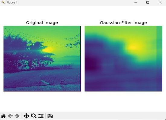
使用高斯核进行卷积
在Mahotas中,高斯核是一个小的数字矩阵,用于模糊或平滑图像。
高斯核对每个像素应用加权平均值,其中权重由称为高斯分布的钟形曲线决定。该核对附近的像素赋予更高的权重,对较远的像素赋予较低的权重。此过程有助于减少噪声并增强图像中的特征,从而产生更平滑、更赏心悦目的输出。
以下是Mahotas中高斯核的基本语法:
mahotas.gaussian_filter(array, sigma)
其中,
array - 输入数组。
sigma - 高斯核的标准差。
示例
以下是使用高斯滤波器对图像进行卷积的示例。在这里,我们正在调整图像大小,将其转换为灰度图像,应用高斯滤波器来模糊图像,然后并排显示原始图像和模糊图像:
import mahotas as mh
import matplotlib.pyplot as mtplt
# Load the image
image = mh.imread('sun.png')
# Convert to grayscale if needed
if len(image.shape) > 2:
   image = mh.colors.rgb2gray(image)
# Resize the image to 128x128
image = mh.imresize(image, (128, 128))
# Create the Gaussian kernel
kernel = mh.gaussian_filter(image, 1.0)
# Reduce the size of the kernel to 20x20
kernel = kernel[:20, :20]
# Blur the image
blurred_image = mh.convolve(image, kernel)
# Creating a figure and subplots
fig, axes = mtplt.subplots(1, 2)
# Displaying original image
axes[0].imshow(image)
axes[0].axis('off')
axes[0].set_title('Original Image')
# Displaying blurred image
axes[1].imshow(blurred_image)
axes[1].axis('off')
axes[1].set_title('Gaussian Filter Image')
# Adjusting the spacing and layout
mtplt.tight_layout()
# Showing the figure
mtplt.show()
输出
上述代码的输出如下:
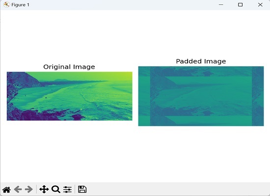
带填充的卷积
Mahotas中的带填充的卷积是指在执行卷积运算之前,在图像边缘周围添加额外的像素或边界。填充的目的是创建一个尺寸更大的新图像,而不会丢失原始图像边缘的信息。
填充确保可以将卷积核应用于所有像素,包括边缘处的像素,从而产生与原始图像大小相同的卷积输出。
示例
在这里,我们定义了一个自定义卷积核作为NumPy数组,以强调图像的边缘:
import numpy as np
import mahotas as mh
import matplotlib.pyplot as mtplt
# Create a custom kernel
kernel = np.array([[0, -1, 0],[-1, 5, -1],
[0, -1, 0]])
# Load the image
image = mh.imread('sea.bmp', as_grey=True)
# Add padding to the image
padding = np.pad(image, 150, mode='wrap')
# Perform convolution with padding
padded_image = mh.convolve(padding, kernel)
# Creating a figure and subplots
fig, axes = mtplt.subplots(1, 2)
# Displaying original image
axes[0].imshow(image)
axes[0].axis('off')
axes[0].set_title('Original Image')
# Displaying padded image
axes[1].imshow(padded_image)
axes[1].axis('off')
axes[1].set_title('Padded Image')
# Adjusting the spacing and layout
mtplt.tight_layout()
# Showing the figure
mtplt.show()
输出
执行上述代码后,我们将得到以下输出:
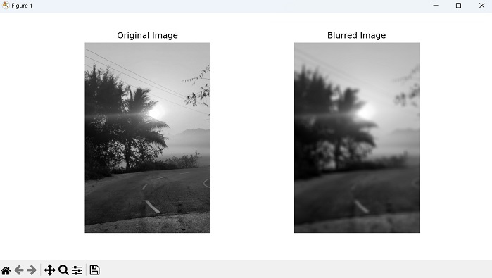
使用盒式滤波器进行模糊处理的卷积
Mahotas中使用盒式滤波器进行卷积是一种可用于模糊图像的技术。盒式滤波器是一个简单的滤波器,其中滤波器核中的每个元素都具有相同的值,从而产生均匀的权重分布。
使用盒式滤波器进行卷积包括将核滑过图像并取核覆盖区域内像素值的平均值。然后,使用该平均值替换输出图像中的中心像素值。
对图像中的所有像素重复此过程,从而产生原始图像的模糊版本。模糊的程度由核的大小决定,较大的核产生更大的模糊。
示例
以下是使用盒式滤波器进行卷积以模糊图像的示例:
import mahotas as mh
import numpy as np
import matplotlib.pyplot as plt
# Load the image
image = mh.imread('sun.png', as_grey=True)
# Define the size of the box filter
box_size = 25
# Create the box filter
box_filter = np.ones((box_size, box_size)) / (box_size * box_size)
# Perform convolution with the box filter
blurred_image = mh.convolve(image, box_filter)
# Display the original and blurred images
fig, axes = plt.subplots(1, 2, figsize=(10, 5))
axes[0].imshow(image, cmap='gray')
axes[0].set_title('Original Image')
axes[0].axis('off')
axes[1].imshow(blurred_image, cmap='gray')
axes[1].set_title('Blurred Image')
axes[1].axis('off')
plt.show()
输出
我们将得到如下所示的输出:
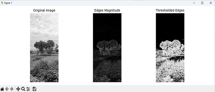
使用Sobel滤波器进行边缘检测的卷积
Sobel滤波器通常用于边缘检测。它由两个单独的滤波器组成:一个用于检测水平边缘,另一个用于检测垂直边缘。
通过将Sobel滤波器与图像进行卷积,我们得到一幅新的图像,其中边缘被突出显示,图像的其余部分显得模糊。与周围区域相比,突出显示的边缘通常具有更高的强度值。
示例
在这里,我们通过将Sobel滤波器与灰度图像进行卷积来执行边缘检测。然后,我们计算边缘的幅度并应用阈值以获得检测到的边缘的二值图像:
import mahotas as mh
import numpy as np
import matplotlib.pyplot as plt
image = mh.imread('nature.jpeg', as_grey=True)
# Apply Sobel filter for horizontal edges
sobel_horizontal = np.array([[1, 2, 1],
[0, 0, 0],[-1, -2, -1]])
# convolving the image with the filter kernels
edges_horizontal = mh.convolve(image, sobel_horizontal)
# Apply Sobel filter for vertical edges
sobel_vertical = np.array([[1, 0, -1],[2, 0, -2],[1, 0, -1]])
# convolving the image with the filter kernels
edges_vertical = mh.convolve(image, sobel_vertical)
# Compute the magnitude of the edges
edges_magnitude = np.sqrt(edges_horizontal**2 + edges_vertical**2)
# Threshold the edges
threshold = 50
thresholded_edges = edges_magnitude > threshold
# Display the original image and the detected edges
fig, axes = plt.subplots(1, 3, figsize=(12, 4))
axes[0].imshow(image, cmap='gray')
axes[0].set_title('Original Image')
axes[0].axis('off')
axes[1].imshow(edges_magnitude, cmap='gray')
axes[1].set_title('Edges Magnitude')
axes[1].axis('off')
axes[2].imshow(thresholded_edges, cmap='gray')
axes[2].set_title('Thresholded Edges')
axes[2].axis('off')
plt.tight_layout()
plt.show()
输出
获得的输出如下: