Mahotas——图像离心率

---

---

图像的离心率是指衡量图像中物体或区域形状拉长或伸展程度的指标。它定量地衡量形状与完美圆形的偏离程度。

离心率的值介于0和1之间，其中：

• 0——表示完美的圆形。离心率为0的物体拉长程度最小，并且完全对称。

• 接近1——表示形状越来越细长。随着离心率值接近1，形状变得越来越细长，越来越不圆。

Mahotas中的图像离心率

我们可以使用'mahotas.features.eccentricity()'函数在Mahotas中计算图像的离心率。

如果离心率值较高，则表明图像中的形状更加拉长或伸展。另一方面，如果离心率值较低，则表明形状更接近于完美的圆形或拉长程度较小。

mahotas.features.eccentricity() 函数

Mahotas中的eccentricity()函数帮助我们测量图像中形状的拉长或伸展程度。此函数将单通道图像作为输入，并返回0到1之间的浮点数。

语法

以下是Mahotas中eccentricity()函数的基本语法：

mahotas.features.eccentricity(bwimage)

其中，'bwimage'是解释为布尔值的输入图像。

示例

在下面的示例中，我们正在查找图像的离心率：

import mahotas as mh
import numpy as np
from pylab import imshow, show
image = mh.imread('nature.jpeg', as_grey = True)
eccentricity= mh.features.eccentricity(image)
print("Eccentricity of the image =", eccentricity)

输出

上述代码的输出如下：

Eccentricity of the image = 0.8902515127811386

使用二值图像计算离心率

为了将灰度图像转换为二值格式，我们使用一种称为阈值化的技术。此过程帮助我们将图像分成两部分：前景（白色）和背景（黑色）。

我们通过选择一个阈值（指示像素强度）来实现这一点，该阈值充当截止点。

Mahotas通过提供“>”运算符简化了这一过程，该运算符允许我们将像素值与阈值进行比较并创建二值图像。准备好二值图像后，我们现在可以计算离心率。

示例

在这里，我们尝试计算二值图像的离心率：

import mahotas as mh
image = mh.imread('nature.jpeg', as_grey=True)
# Converting image to binary based on a fixed threshold
threshold = 128
binary_image = image > threshold
# Calculating eccentricity
eccentricity = mh.features.eccentricity(binary_image)
print("Eccentricity:", eccentricity)

输出

执行上述代码后，我们将得到以下输出：

Eccentricity: 0.7943319646935899

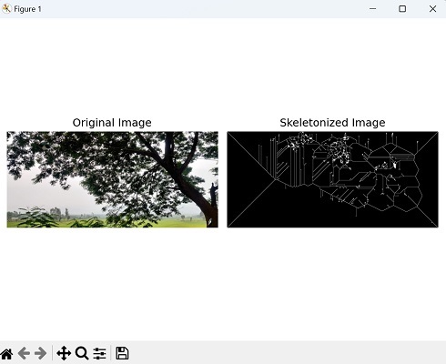
使用细化计算离心率

细化，也称为细化，是一个旨在减少物体形状或结构的过程，将其表示为细长的骨架。我们可以使用Mahotas中的thin()函数来实现这一点。

mahotas.thin()函数将二值图像作为输入，其中感兴趣的物体由白色像素（像素值为1）表示，背景由黑色像素（像素值为0）表示。

我们可以通过将图像简化为其骨架表示来使用细化计算图像的离心率。

示例

现在，我们使用细化计算图像的离心率：

import mahotas as mh
import matplotlib.pyplot as plt
# Read the image and convert it to grayscale
image = mh.imread('tree.tiff')
grey_image = mh.colors.rgb2grey(image)
# Skeletonizing the image
skeleton = mh.thin(grey_image)
# Calculating the eccentricity of the skeletonized image
eccentricity = mh.features.eccentricity(skeleton)
# Printing the eccentricity
print(eccentricity)
# Create a figure with subplots
fig, axes = plt.subplots(1, 2, figsize=(7,5 ))
# Display the original image
axes[0].imshow(image)
axes[0].set_title('Original Image')
axes[0].axis('off')
# Display the skeletonized image
axes[1].imshow(skeleton, cmap='gray')
axes[1].set_title('Skeletonized Image')
axes[1].axis('off')
# Adjust the layout and display the plot
plt.tight_layout()
plt.show()

输出

获得的输出如下所示：

0.8975030064719701

显示的图像是如下所示：